Understanding PyTorch with an example: a step-by-step tutorial
a linear regression with a single feature x
y = a + bx + εLet’s start generating some synthetic data: 100 points for our feature x and create our labels ,
using a = 1, b = 2 and some Gaussian noise.
Next, let’s split our synthetic data into train and validation sets, shuffling the array of indices and using the first 80 shuffled points for training.
def data_gen():
    # Data Generation
    np.random.seed(42)

    a,b = 1,2
    x = np.random.rand(100, 1)
    y = a + b * x + .1 * np.random.randn(100, 1)

    # Shuffles the indices
    idx = np.arange(100)
    np.random.shuffle(idx)

    # Uses first 80 random indices for train
    train_idx = idx[:80]
    # Uses the remaining indices for validation
    val_idx = idx[80:]

    # Generates train and validation sets
    x_train, y_train = x[train_idx], y[train_idx]
    x_val, y_val = x[val_idx], y[val_idx]

    return x_train, y_train , x_val, y_val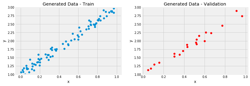
| data from | data to | method | comments |
|---|---|---|---|
| numpy | cpu tensor | from_numpy() | |
| cpu tensor | gpu tensor | to() | cuda.is_available() to find out whether you have a GPU |
| cpu tensor | to float32 | float() | |
| cpu tensor | numpy | numpy() | you can convert CUDA(GPU) tensor to numpy |
| gpu tensor | cpu tensor | cpu() |
import torch
import torch.optim as optim
import torch.nn as nn
from torchviz import make_dot

device = 'cuda' if torch.cuda.is_available() else 'cpu'

# Our data was in Numpy arrays, but we need to transform them into PyTorch's Tensors
# and then we send them to the chosen device
x_train_tensor = torch.from_numpy(x_train).float().to(device)
y_train_tensor = torch.from_numpy(y_train).float().to(device)

# Here we can see the difference - notice that .type() is more useful
# since it also tells us WHERE the tensor is (device)
print(type(x_train), type(x_train_tensor), x_train_tensor.type())
# <class 'numpy.ndarray'> <class 'torch.Tensor'> torch.FloatTensor- Initializes parameters "a" and "b" randomly
- set
requires_grad=Truetells PyTorch we want it to compute gradients for us.
a = torch.randn(1, requires_grad=True, dtype=torch.float)
b = torch.randn(1, requires_grad=True, dtype=torch.float)
print(a, b)
# tensor([-0.5836], requires_grad=True) tensor([-0.7957], requires_grad=True)
- Q(todo): requires_grad is a flag, defaulting to false unless wrapped in a
nn.Parameter?
- set
- if we want to run it on a GPU
a = torch.randn(1, dtype=torch.float).to(device)
b = torch.randn(1, dtype=torch.float).to(device)
# and THEN set them as requiring gradients...
a.requires_grad_()
b.requires_grad_()
- or specify the device at the moment of creation -- RECOMMENDED!
a = torch.randn(1, requires_grad=True, dtype=torch.float, device=device)
b = torch.randn(1, requires_grad=True, dtype=torch.float, device=device)
In PyTorch, every method that ends with an underscore (_) makes changes in-place, meaning, they will modify the underlying variable.
- how do we tell PyTorch to do "auto-grad" ?
- backward()
- invoke
loss.backward()
- What about the actual values of the gradients?
- We can inspect them by looking at the grad attribute of a tensor.
- PS. the gradients are accumulated
- So, every time we use the gradients to update the parameters, we need to zero the gradients afterwards.
- zero_()
    lr = 1e-1
    n_epochs = 1000

    torch.manual_seed(42)
    a = torch.randn(1, requires_grad=True, dtype=torch.float, device=device)
    b = torch.randn(1, requires_grad=True, dtype=torch.float, device=device)

    for epoch in range(n_epochs):
        yhat = a + b * x_train_tensor
        error = y_train_tensor - yhat
        loss = (error ** 2).mean()

        # No more manual computation of gradients!
        # a_grad = -2 * error.mean()
        # b_grad = -2 * (x_tensor * error).mean()

        # We just tell PyTorch to work its way BACKWARDS from the specified loss!
        loss.backward()
        # Let's check the computed gradients...
        print(a.grad)
        print(b.grad)

        # What about UPDATING the parameters? Not so fast...

        # FIRST ATTEMPT
        # AttributeError: 'NoneType' object has no attribute 'zero_'
        #   reassigning the update results to our parameters lost the gradient
        # a = a - lr * a.grad
        # b = b - lr * b.grad
        # print(a)

        # SECOND ATTEMPT
        # RuntimeError: a leaf Variable that requires grad has been used in an in-place operation.
        #   python is gonna build a dynamic computation graph from every Python operation
        #   that involves any gradient-computing tensor or its dependencies.
        # a -= lr * a.grad
        # b -= lr * b.grad

        # THIRD ATTEMPT
        # We need to use NO_GRAD to keep the update out of the gradient computation
        # Why is that? It boils down to the DYNAMIC GRAPH that PyTorch uses...
        #   no_grad() allows us to perform regular Python operations on tensors,
        #   independent of PyTorch’s computation graph.
        with torch.no_grad():
            a -= lr * a.grad
            b -= lr * b.grad

        # PyTorch is "clingy" to its computed gradients, we need to tell it to let it go...
        a.grad.zero_()
        b.grad.zero_()

    print(a, b)

# tensor([1.0235], requires_grad=True) tensor([1.9690], requires_grad=True)PyTorchViz package and its make_dot(variable) method allows us to easily visualize a graph associated with a given Python variable.
from torchviz import make_dot
...

make_dot(yhat)So far, we’ve been manually updating the parameters using the computed gradients.
That’s probably fine for two parameters… but what if we had a whole lot of them?!
We use one of PyTorch’s optimizers, like SGD or Adam.
- An optimizer takes
- the parameters we want to update,
- the learning rate we want to use, (and possibly many other hyper-parameters as well!)
- and performs the updates through its step() method.
Besides, we also don’t need to zero the gradients one by one anymore. We just invoke the optimizer’s zero_grad() method and that’s it!
    torch.manual_seed(42)
    # parameters
    a = torch.randn(1, requires_grad=True, dtype=torch.float, device=device)
    b = torch.randn(1, requires_grad=True, dtype=torch.float, device=device)

    lr = 1e-1
    n_epochs = 1000

    # Defines a SGD optimizer to update the parameters
    optimizer = optim.SGD([a, b], lr=lr)

    for epoch in range(n_epochs):
        yhat = a + b * x_train_tensor
        error = y_train_tensor - yhat
        loss = (error ** 2).mean()

        loss.backward()

        # No more manual update!
        # with torch.no_grad():
        #     a -= lr * a.grad
        #     b -= lr * b.grad
        optimizer.step()

        # No more telling PyTorch to let gradients go!
        # a.grad.zero_()
        # b.grad.zero_()
        optimizer.zero_grad()

print(a, b) loss = (error ** 2).mean()We now tackle the loss computation. As expected, PyTorch got us covered once again. There are many loss functions to choose from, depending on the task at hand.
Since ours is a regression, we are using the Mean Square Error (MSE) loss. nn.MSELoss.
Notice that nn.MSELoss actually creates a loss function for us — it is NOT the loss function itself. Moreover, you can specify a reduction method to be applied, that is, how do you want to aggregate the results for individual points — you can average them (reduction=’mean’) or simply sum them up (reduction=’sum’).
    torch.manual_seed(42)
    a = torch.randn(1, requires_grad=True, dtype=torch.float, device=device)
    b = torch.randn(1, requires_grad=True, dtype=torch.float, device=device)
    print(a, b)

    lr = 1e-1
    n_epochs = 1000

    # Defines a MSE loss function
    loss_fn = nn.MSELoss(reduction='mean')

    optimizer = optim.SGD([a, b], lr=lr)

    for epoch in range(n_epochs):
        yhat = a + b * x_train_tensor

        # No more manual loss!
        # error = y_tensor - yhat
        # loss = (error ** 2).mean()
        loss = loss_fn(y_train_tensor, yhat)

        loss.backward()
        optimizer.step()
        optimizer.zero_grad()

    print(a, b)
At this point, there’s only one piece of code left to change: the predictions. It is then time to introduce PyTorch’s way of implementing a…
In PyTorch, a model is represented by a regular Python class that inherits from the Model class
__init__(self)- it defines the parts that make up the model
- in our case, two parameters, a and b.
- forward(self, x)
- it performs the actual computation, that is, it outputs a prediction, given the input x.
- You should NOT call the forward(x) method. You should call the whole model itself,
model(x).
Let’s build a proper (yet simple) model
class ManualLinearRegression(nn.Module):
    def __init__(self):
        super().__init__()
        # To make "a" and "b" real parameters of the model, we need to wrap them with nn.Parameter
        self.a = nn.Parameter(torch.randn(1, requires_grad=True, dtype=torch.float))
        self.b = nn.Parameter(torch.randn(1, requires_grad=True, dtype=torch.float))

    def forward(self, x):
        # Computes the outputs / predictions
        return self.a + self.b * x
Moreover, we can get the current values for all parameters using our model’s state_dict() method.
IMPORTANT: we need to send our model to the same device where the data is. If our data is made of GPU tensors, our model must “live” inside the GPU as well.
    # training
    torch.manual_seed(42)

    # Now we can create a model and send it at once to the device
    model = ManualLinearRegression().to(device)
    # We can also inspect its parameters using its state_dict
    print(model.state_dict())

    lr = 1e-1
    n_epochs = 1000

    loss_fn = nn.MSELoss(reduction='mean')
    # parameters() instead of a,b
    optimizer = optim.SGD(model.parameters(), lr=lr)

    for epoch in range(n_epochs):
        # What is this?!?
        # does NOT perform a training step
        # Its only purpose is to set the model to training mode.
        # Some models may use mechanisms like Dropout, for instance,
        #   which have distinct behaviors in training and evaluation phases.
        model.train()

        # No more manual prediction!
        # yhat = a + b * x_tensor
        yhat = model(x_train_tensor)

        loss = loss_fn(y_train_tensor, yhat)
        loss.backward()
        optimizer.step()

    print(model.state_dict())

# OrderedDict([('a', tensor([0.3367])), ('b', tensor([0.1288]))])
# OrderedDict([('a', tensor([1.0235])), ('b', tensor([1.9690]))])
Full Code
#!python3
import numpy as np

import torch
import torch.optim as optim
import torch.nn as nn
# from torchviz import make_dot
import torchvision


class ManualLinearRegression(nn.Module):
    def __init__(self):
        super().__init__()
        # To make "a" and "b" real parameters of the model, we need to wrap them with nn.Parameter
        self.a = nn.Parameter(torch.randn(1, requires_grad=True, dtype=torch.float))
        self.b = nn.Parameter(torch.randn(1, requires_grad=True, dtype=torch.float))

    def forward(self, x):
        # Computes the outputs / predictions
        return self.a + self.b * x

def data_gen():
    # Data Generation
    np.random.seed(42)

    a,b = 1,2
    x = np.random.rand(100, 1)
    y = a + b * x + .1 * np.random.randn(100, 1)

    # Shuffles the indices
    idx = np.arange(100)
    np.random.shuffle(idx)

    # Uses first 80 random indices for train
    train_idx = idx[:80]
    # Uses the remaining indices for validation
    val_idx = idx[80:]

    # Generates train and validation sets
    x_train, y_train = x[train_idx], y[train_idx]
    x_val, y_val = x[val_idx], y[val_idx]

    return x_train, y_train , x_val, y_val

def show_data( x, y ):
    # import matplotlib.pyplot as plt
    # plt.scatter( x,y )
    # plt.show()
    pass


if __name__ == '__main__':
    x_train, y_train , x_val, y_val = data_gen()
    show_data( x_train, y_train )

    device = 'cuda' if torch.cuda.is_available() else 'cpu'

    # Our data was in Numpy arrays, but we need to transform them into PyTorch's Tensors
    # and then we send them to the chosen device
    x_train_tensor = torch.from_numpy(x_train).float().to(device)
    y_train_tensor = torch.from_numpy(y_train).float().to(device)

    # Here we can see the difference - notice that .type() is more useful
    # since it also tells us WHERE the tensor is (device)
    print(type(x_train), type(x_train_tensor), x_train_tensor.type())

    # training
    torch.manual_seed(42)

    # Now we can create a model and send it at once to the device
    model = ManualLinearRegression().to(device)
    # We can also inspect its parameters using its state_dict
    print(model.state_dict())

    lr = 1e-1
    n_epochs = 1000

    loss_fn = nn.MSELoss(reduction='mean')
    # parameters() instead of a,b
    optimizer = optim.SGD(model.parameters(), lr=lr)

    for epoch in range(n_epochs):
        # What is this?!?
        model.train()

        # No more manual prediction!
        # yhat = a + b * x_tensor
        yhat = model(x_train_tensor)

        loss = loss_fn(y_train_tensor, yhat)
        loss.backward()
        optimizer.step()
        optimizer.zero_grad()

print(model.state_dict())In our model, we manually created two parameters to perform a linear regression.
Let’s use PyTorch’s Linear model as an attribute of our own, thus creating a nested model. Even though this clearly is a contrived example...
class LayerLinearRegression(nn.Module):
    def __init__(self):
        super().__init__()
        # Instead of our custom parameters, we use a Linear layer with single input and single output
        self.linear = nn.Linear(1, 1)

    def forward(self, x):
        # Now it only takes a call to the layer to make predictions
return self.linear(x)For straightforward models, that use run-of-the-mill layers, where the output of a layer is sequentially fed as an input to the next, we can use a, er… Sequential model :-)
    # Alternatively, you can use a Sequential model
model = nn.Sequential(nn.Linear(1, 1)).to(device)So far, we’ve defined an optimizer, a loss function and a model.
Would the code inside for-loop change if we were using a different optimizer, or loss, or even model? If not, how can we make it more generic?
So, how about writing a function that takes those three elements and returns another function that performs a training step, taking a set of features and labels as arguments and returning the corresponding loss?
def make_train_step(model, loss_fn, optimizer):
    # Builds function that performs a step in the train loop
    def train_step(x, y):
        # mostly a copy from code inside for-loop
        # Sets model to TRAIN mode
        model.train()
        # Makes predictions
        yhat = model(x)
        # Computes loss
        loss = loss_fn(y, yhat)
        # Computes gradients
        loss.backward()
        # Updates parameters and zeroes gradients
        optimizer.step()
        optimizer.zero_grad()
        # Returns the loss
        return loss.item()

    # Returns the function that will be called inside the train loop
    return train_step

# Creates the train_step function for our model, loss function and optimizer
train_step = make_train_step(model, loss_fn, optimizer)
losses = []

# For each epoch...
for epoch in range(n_epochs):
    # Performs one train step and returns the corresponding loss
    loss = train_step(x_train_tensor, y_train_tensor)
    losses.append(loss)

# Checks model's parameters
print(model.state_dict())PyTorch’s random_split() method is an easy and familiar way of performing a training-validation split.
from torch.utils.data.dataset import random_split

x_tensor = torch.from_numpy(x).float()
y_tensor = torch.from_numpy(y).float()

dataset = TensorDataset(x_tensor, y_tensor)

train_dataset, val_dataset = random_split(dataset, [80, 20])

train_loader = DataLoader(dataset=train_dataset, batch_size=16)
val_loader = DataLoader(dataset=val_dataset, batch_size=20)This is the last part of our journey , we need to change the training loop to include the evaluation of our model, that is, computing the validation loss.
losses = []
val_losses = []
train_step = make_train_step(model, loss_fn, optimizer)

for epoch in range(n_epochs):
    for x_batch, y_batch in train_loader:
        x_batch = x_batch.to(device)
        y_batch = y_batch.to(device)

        loss = train_step(x_batch, y_batch)
        losses.append(loss)

    with torch.no_grad():  # 1
        for x_val, y_val in val_loader:
            x_val = x_val.to(device)
            y_val = y_val.to(device)

            model.eval()

            yhat = model(x_val)
            val_loss = loss_fn(y_val, yhat)
            val_losses.append(val_loss.item())

print(model.state_dict())
there are two small, yet important, things to consider:
torch.no_grad()- even though it won’t make a difference in our simple model, it is a good practice to wrap the validation inner loop with this context manager to disable any gradient calculation that you may inadvertently trigger
- gradients belong in training, not in validation steps;
- eval()
- the only thing it does is setting the model to evaluation mode (just like its train() counterpart did)
- so the model can adjust its behavior regarding some operations, like Dropout.